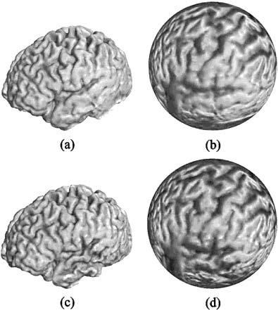
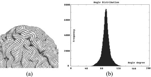
The algorithm uses covariant differentiation to solve a geometric nonlinear partial differential equation (PDE). The complexity of the algorithm is , where is the number of the vertices of the brain mesh, is the number of required iterations. mainly depends on the initial condition, i.e., how close it is to<br />a conformal map. also depends on the step length. Table II illustrates the CPU time for computing conformal maps of surfaces of different triangle numbers on a 1.9-GHz PC with the Windows XP operating system.<br /><br />Comparing to other algorithms that solve a linear system, our nonlinear algorithm has the following unique advantages. First, every point on the brain is treated in a uniform way—no point maps to infinity. Therefore, there are no specific areas with large distortion. Second, the method is very general, as it does not require the target surface to be a sphere. It can be easily generalized to compute harmonic maps between any two arbitrary genus zero surfaces.<br />The 3-D brain meshes are reconstructed from 3-D 256 256 124 T1 weighted SPGR (spoiled gradient) MRI images, by using an active surface algorithm that deforms a triangulated mesh onto the brain surface . Fig. 1 shows the same brain scanned at different times. Because of the inaccuracy introduced by scanner noise in the input data, as well as slight biological changes over time, the geometric information is not exactly the same. Fig. 1 reveals minor differences.<br />The conformal mapping results are shown in Fig.2. From this example, we can see that although the brain meshes are slightly different, the mapping results look quite similar.<br /><br />Figure 1: Reconstructed brain meshes and their spherical harmonic mappings and (c) are the reconstructed surfaces for the same brain scanned at different times. Due to scanner noise and inaccuracy in the reconstruction algorithm, there are visible geometric differences. (b) and (d) are the spherical conformal mappings of (a) and (c), respectively; the normal information is preserved. By the shading information, the correspondence is illustrated<br /><br />Figure 2: Conformality measurement. (a) Intersection angles; (b) Angle distribution. The curves of iso-polar angle and iso-azimuthal angle are mapped to the brain, and the intersection angles are measured on the brain. The histogram is illustrated.